PID Control in Flowcode

PID control is used extensively in industry to control machinery and maintain working environments etc. The fundamentals of PID control are fairly straightforward, but implementing them in practise can prove to be a uphill struggle. In this article we provide a clear explanation of how PID control works and also a couple of Flowcode example files designed to demonstrate how PID control is performed.

Proportional Integral Derivative (PID) Control

When controlling a real system such as a motor there is normally an error between the speed you wish to drive the motor and the speed the motor is running. This is due in part to the fact that the motor will take time to respond and also due to the fact that the load on the motor can change. Adding some kind of feedback to the system allows us to essentially close the loop allowing us to control the motor, read the feedback and then adjust our output signal to suit.

PID control is essentially a mechanism that is used to monitor and control a varying system, for example when we are driving along in a car our brain is automatically tracking the distance from the central line and adjusting accordingly. This type of system is known as a closed loop system as we do an action such as turn the steering wheel then monitor the response by looking at the road and then adjusting the steering wheel if necessary.

Example of closed loop system using PID

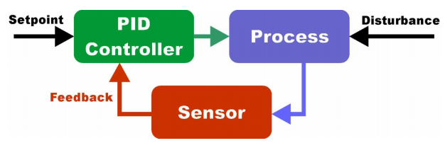
The above diagram contains some terms, here are the definitions:

Setpoint – Desired output of the system.

PID Controller – System monitoring setpoint and feedback eg the brain or a microcontroller.

Output –The modified output from the controller.

Process – The action that is happening eg driving along the road.

Disturbances – Outside influences on the system eg turns in the road.

Sensor – A way of measuring how far off our setpoint we are eg our eyes.

Feedback – The control signal fed into the controller from the sensor.

The PID equation is used a lot in control systems as it takes into account three types of feedback error.

• Proportional error – This is the simplest form of error and simply tells us the difference between the setpoint and the feedback signal.
• Integral error – This is used to correct any end result offset that the proportional control cannot reduce due to gain limitations by creating a rolling average of previous errors.
• Derivative error – This uses multiple errors over time to monitor the rate of change and try to predict what is going to happen next.

The basic PID function is basically a sum of all three types of error.

Output = Pout + Iout + Dout

An example of the PID equation using three previous error readings would look like this.

Output = P * (Error – Prev_Error + (Error / I) + D * (Error – (2 * Prev_Error) + Prev_Prev_Error))

To calculate the errors in the above equation we are basically subtracting the sensor feedback from the control setpoint. To allow this to work effectively there has to be a way of allowing the feedback signal to be equal to the setpoint. This way when both the setpoint and the feedback match the error is zero.

Here is a worked example of the above equation;

Setpoint = 5

P = 2

I = 6

D = 1

(Step 1)

Feedback = 0

P * (5 – 5 + (5 / I) + D * (5 – (2 * 5) + 5)) = 10

At step 1 we are far from the setpoint so we have a large output to try and speed up the process to get to the setpoint.

(Step 2)

Feedback = 1

P * (4 – 5 + (4 / I) + D * (4 – (2 * 5) + 5)) = -2.66

At step 2 we are predicting that the setpoint will shortly be reached so we are backing off the control signal slightly from 10 to 7.34.

(Step 3)

Feedback = 2

P * (3 – 4 + (3 / I) + D * (3 – (2 * 4) + 5)) = -1

At step 3 we are nearing the setpoint so the control signal tries to back off more to avoid overshooting the setpoint and changes from 7.34 to 6.34.

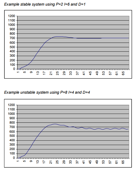
A system controlled by PID requires tuning to make the system stable and achieve the fastest possible response to the control signal. To aid in this we have generated an Excel spreadsheet that simulates a second order system such as a DC motor. Different values for the P, I and D control values can be tested and the starting point and setpoint can be altered for any given situation. It is normally fairly simple to see if a system is going to respond well or become unstable as long as you have the system characteristics modelled correctly.Tuning a system can often be fairly hard to do without loads of trial and error. There are ways to allow the PID system to tune itself but these systems are often said to be teetering on the unstable side and the slightest unpredicted error can cause lots of problems.

A reactive PID system should aim for a little overshoot before settling down. Rule of thumb values are that P is roughly equal to I and D is roughly one quarter the value of I.

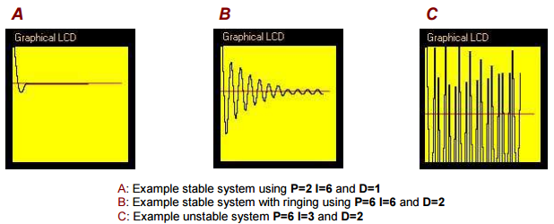
The first example uses my integer based PID calculation to simulate this second order system on hardware. To do this I am using the EB064 – dsPIC and PIC24 Multiprogrammer E-block along with a EB058 graphical LCD. The program creates a random setpoint between 0 and 100 which it draws as a red line and then plots the response of the PID algorithm. Here we can see the differences between our excel calculation and our microcontroller based integer only calculation. It should be possible to see that the discrete sampled system is a lot more prone to becoming unstable due to fractional errors in the equation.

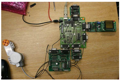
Now that we can simulate a PID control signal how about applying it in practise. To do this I am using a new style NXP Lego DC motor but the same method can be applied to just about any system that can be effected by the surroundings with outputs that can be measured, e.g. room temperature, motor speed, motor position, generator output, voltage charge pumps etc.

The next example shows how to apply the PID algorithm by using actual feedback to control the error signals rather than using a simulated error. To start you first need to determine the range of your control signal. I will be using PWM to control the speed of a Lego DC motor. The PWM input is a byte so this can go between 0 and 255 where 0 is the motor is stopped and 255 is the motor at full speed. To feed error back into the system I will be using the opto-encoder fitted inside the motor to measure its speed. Again I will let the program pick random setpoints and plot the response of the algorithm onto the graphical display. The running program controls the motor and will try to maintain a steady speed to match the setpoint even if the load on the motor changes significantly.

The feedback signal from the Lego motor is fairly good, but not amazing, and therefore the control of the motor is not perfect. However, it is obviously far better than using normal open loop control. Using a shaft encoder with a greater resolution would allow for a better motor response. To get the encoder feedback to approximately equal the setpoint to generate a 0 error I have measured the encoder response when the motor is at full speed. Doing this I found that a speed of 255 represented an encoder frequency of around 125 cycles in 25ms. Therefore to normalise the feedback signal I simply multiplied it by 2 before calculating the error and then plugging this into the PID equation which runs every 25ms.

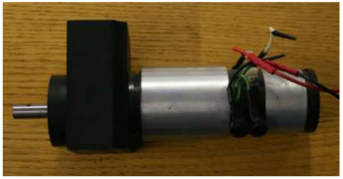
This motor was taken from a industrial robotic camera and uses a tacho as the source of feedback rather than an encoder. The tacho gives us an analogue signal that is proportional to the rotational speed of the motor. So to monitor the error from a motor like this a potential divider circuit would be used to get the tacho signal as close as possible to the control signal when read in through an ADC.

The examples in this article were written for the dsPIC30F2011 device that comes as standard with the EB064 PIC24 and dsPIC E-block. The PID algorithm also could be improved by using floating point calculations rather than integer based calculations though this would have an impact on the speed of the PID routine as well as the amount of code that is generated. In practise the integer based PID algorithm is working well.

You can download the simulatable PID routine for Flowcode here.

12,828 total views, 1 views today